A Step-by-Step Guide to Using a Naïve Bayes Classifier to Predict the Direction of Apple Stock in R.

Now that we have an understanding of the basic concepts of using machine-learning algorithms in your strategy (you can find the first part of the series here), we’ll go through a basic example of how to use a Naïve Bayes classifier to predict the direction of Apple stock. First, we will gather a basic understanding of how a Naïve Bayes classifier works, then we will step through a very simple example using the day of the week to predict whether the day’s price will close up or down, and finally we will build a more sophisticated model adding a technical indicator.

What is a Naïve Bayes classifier?

A Naïve Bayes classifier tries to find the probability that A will happen given that B has already occurred, commonly denoted by P(A | B) (the probability of A given B).

For our case, we are basically asking “what is the probability that today’s price will increase given that today is Wednesday?” The Naïve Bayes looks at both the overall probability that today’s price will increase, i.e. the number of days the price has closed up over the total number of days, and the probability that today’s price will increase given that today is Wednesday, i.e. on how many previous Wednesdays did the price close up?

We are then able to compare the probability that today’s price will increase to the probability it will decrease, and choose the case with the higher probability as our prediction.

So far we have only been talking about including one indicator, but as multiple indicators are included, the math quickly becomes very complicated. To get around this, the Naïve Bayes treats every indicator as independent, or uncorrelated (hence the term Naïve). So it is important to choose indicators that are uncorrelated over indicators that may be telling you the same information. In practice, the Naïve Bayes isn’t great at learning relationships between your indicators (such as, when it is Tuesday AND the RSI is above 75, there is an exceptionally high probability the next day’s price will be down) but it does perform reasonably well even if there is some correlation among your indicators.

This is a very simplified, high-level overview of the Naïve Bayes but should give you a basic understanding of how it works. If you would like to learn more about the Naïve Bayes and other machine-learning algorithms, here is a great source.

Step-By-Step Example in R

Now we will go through a very simple example in R. We will use the day of the week to predict whether today’s price of Apple stock will close up or down.

First, let’s make sure we have all the libraries we need installed and loaded.

						install.packages("quantmod")


						library("quantmod")


						#Allows us to import the data we need

					

						install.packages("lubridate")


						library("lubridate")


						#Makes it easier to work with the dates

					

						install.packages("e1071")


						library("e1071")


						#Gives us access to the Naïve Bayes classifier
					

Next, let’s get all the data we will need.

						startDate = as.Date("2012-01-01")


						# The beginning of the date range we want to look at

					

						endDate = as.Date("2014-01-01") 


						# The end of the date range we want to look at

					

						getSymbols("AAPL", src = "yahoo", from = startDate, to = endDate) 


						# Retrieving Apple’s daily OHLCV from Yahoo Finance

					

Now that we have all the data we will need, let’s get our indicator, the day of the week.

						DayofWeek<-wday(AAPL, label=TRUE)


						#Find the day of the week

					

And what we are trying to predict, whether the day’s price will close up or down, and create the final data set.

						PriceChange<- Cl(AAPL) - Op(AAPL)


						#Find the difference between the close price and open price

					

						Class<-ifelse(PriceChange>0,"UP","DOWN")


						#Convert to a binary classification. (In our data set, there are no bars with an exactly 0 price change so, for simplicity sake, we will not address bars that had the same open and close price.)

					

						DataSet<-data.frame(DayofWeek,Class)


						#Create our data set

					

Finally, we are ready to use the Naïve Bayes classifier.

						MyModel<-naiveBayes(DataSet[,1],DataSet[,2])


						#The input, or independent variable (DataSet,1]), and what we are trying to predict, the dependent variable (DataSet[,2]).

					

Congratulations! We have now used a machine-learning algorithm to analyze Apple stock. Now, let’s dive into the results.

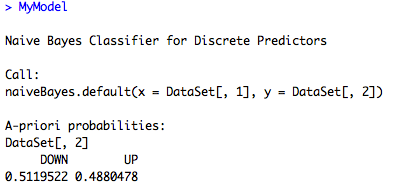This shows us the probability of a price increase or decrease over our entire data set (known as the prior probabilities). We can see there is a slight bearish bias, but not much.

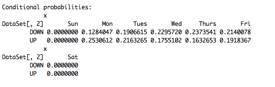This shows the conditional probabilities (Given that it is a certain day of the week, what is the probability that the price will close up or down.) These are much lower than 50% due the fact they are scaled down by the prior probabilities of the outcomes (probability of price increase over the entire data set).

We are able to see that this this not a very good model, i.e. it does not return very high probabilities. However, we can see that you are generally better off going long in the beginning of the week and short towards the end of the week.

Improving the Model

Obviously you are going to want a slightly more sophisticated strategy than just looking at the day of the week. Let’s now add a moving average cross to our model. (You can get some more information on adding other indicators, or features, to your model here.)

I prefer using exponential moving averages, so let’s look at a 5-period and 10-period exponential moving average (EMA) cross.

First, we need to calculate the EMAs:

						EMA5<-EMA(Op(AAPL),n = 5)


						#We are calculating a 5-period EMA off the open price

					

						EMA10<-EMA(Op(AAPL),n = 10)


						#Then the 10-period EMA, also off the open price

					

Then calculate the cross

						EMACross <- EMA5 - EMA10 


						#Positive values correspond to the 5-period EMA being above the 10-period EMA

					

And rounding the values to 2 decimal places. This is important because if there is an instance that the Naïve Bayes has never seen, it will automatically calculate the probability at 0%. For example, if we were looking at the EMA cross to 6 decimal places and it found a very high probability of a downward price movement when the difference was $2.349181 and then was presented with a new data point that had the difference as $2.349182, it would calculate a 0% probability leading to a price increase or decrease. By rounding to 2 decimal places, we greatly mitigate this risk as a large enough dataset it should have seen most values of the indicator. This is an important limitation to remember when building your own models.

						EMACross<-round(EMACross,2)


					

Let’s create a new dataset and split it into a training and test set so we are able to see how well our model does over new data

						DataSet2<-data.frame(DayofWeek,EMACross, Class)


						DataSet2<-DataSet2[-c(1:10),]


						#We need to remove the instances where the 10-period moving average is still being calculated


						TrainingSet<-DataSet2[1:328,]


						#We will use ⅔ of the data to train the model


						TestSet<-DataSet2[329:492,] 


						#And ⅓ to test it on unseen data

					

Now to build the model:

						EMACrossModel<-naiveBayes(TrainingSet[,1:2],TrainingSet[,3])

					

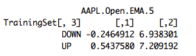The Conditional Probability of the EMA Cross, a numeric variable, shows the mean value for each case ([,1]), and the standard deviation ([,2]). We can see that the mean difference between the 5-period EMA and 10-period EMA for long and short trades was $0.54 and -$0.24, respectively.

And test it over new data:

					table(predict(EMACrossModel,TestSet),TestSet[,3],dnn=list('predicted','actual'))

					

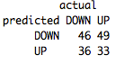We can see overall it got 79 out of 164, or 48%, correct. It had a fairly large downward bias, predicting 95, or 58%, cases as “DOWN”.

While these are not great results, this should give you all the information you need to build your own machine-learning based strategy.

In the next part of our series, we will go over how you can actually use this model to improve your own trading.