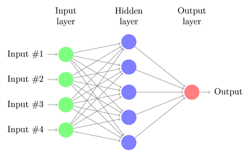
Artificial neural networks are very powerful and popular machine-learning algorithms that mimic how a brain works in order find patterns in your data.

While they can become fairly complex and require tuning a wide variety of parameters, they have the potential to be very effective and should be explored. In this post, we will give a basic introduction to how neural networks work, discuss how to tune the parameters, and build a basic neural network to model the S&P 500. In the next section we will discuss how to optimize the neural network and how to apply the model to your own trading.

Be sure to also check out our posts on Naive Bayes Classifiers and Decisions Trees.

What is an Artificial Neural Network?

Artificial neural networks (ANNs), similar to a brain, consist of a network of interconnected “neurons”. These neurons communicate with each other through a large number of weighted connections. When an incoming signal reaches a certain level, a neuron becomes active based on its “activation function”. Once this neuron is activated, it then passes along its signal to the next level of neurons, with the strength of the signal determined by the weight of each connection.

ANNs make predictions by sending the inputs (in our case, the indicators) through the network of neurons, with the neurons firing off depending on the weights of the incoming signals. The final output is determined by the strength of the signals coming from the previous layer of neurons. While these networks have the benefit of being able to model any arbitrarily complex dataset, many questions remain on how the network should be built. You must decide on the number of layers of neurons (known as “hidden layers”), number of neurons in each layer, how a neuron is activated, and how the weights between neurons change, or learn, over time.

Determining the Parameters of Your Network

One of the most important decisions when using ANNs is to determine the network architecture, or the number of hidden layers and the number of neurons in each layer. The first, or input, layer is set by your number of inputs and the final, or output, layer is determined by the number of outputs (in our case, we are just looking to forecast a single variable; the price direction). This leaves the question of how many hidden layers should I have and how many neurons in each layer should I include? If you have too few hidden layers you won’t be able to model complex patterns in your data and with too many you won’t generalize well over new data. Two hidden layers generally provide enough flexibility to model even highly-complex data sets.

A good rule of thumb for determining the number of neurons to include in each hidden layer is that it should fall somewhere between the number of inputs and number of outputs. However, the best results are often found through “trial-and-error”, where you select the tree architecture with the lowest cross-validated error over your data.

For our example, we will use a neural network of two hidden layers with 3 neurons each.

Now that we have the architecture of our network, we need to figure out when a neuron should be activated. For this example, we will use a logistic sigmoid activation function, a very popular method that allows us to model non-linear data and limits the range of the signals from 0 to 1.

The last step is to figure out how to determine the weights between the neurons. A common method is through “backpropagation”. A neural network attempts to minimize the the squared error between the predicted value and actual value for each data point. The error is minimized through a gradient descent, which can be thought of as taking a step in the direction of the weight that decreases the error (the size of this step is known as the “learning rate”). Backpropagation works backwards from the output layer and adjusts the weights between each neuron by the learning rate until it reaches a local minimum error or a stopping criteria.

We will use a backpropagation algorithm with a learning rate of .001.

There are many more sophisticated parameters and methods to building an ANN, however these are the basic ones you need to know about before moving forward. The best results are usually found by evaluating the parameters over your particular dataset.

Now that we have that taken care of the basic concepts, let’s build our neural network!

Building Your Network

An important thing to remember when using an ANN, especially with a sigmoid activation function, is that you need to normalize your data between 0 and 1.

So let’s first install the libraries we need and build our datasets.

						install.packages("quantmod")

						library("quantmod")

						#Allows us to import the market data and indicators we need
					

						install.packages(“neuralnet”)

						library(“neuralnet”)

						#Provides the artificial neural network algorithm (there are a variety of R packages that allow you build ANNs, however neuralnet allows us to easily plot the network and has all the functionality we need for this example)
					

						startDate<-as.Date('2009-01-01')

						endDate<-as.Date('2014-01-01')

						getSymbols("^GSPC",src="yahoo",from=startDate,to=endDate)

						#Retrieve the data we need
					

						RSI3<-RSI(Op(GSPC),n=3)

						#Calculate a 3-period RSI
					

						EMA5<-EMA(Op(GSPC),n=5)

						EMAcross<-Op(GSPC)-EMA5

						#Look at the difference between the open price and a 5-period EMA
					

						MACD<-MACD(Op(GSPC),fast = 12, slow = 26, signal = 9)

						MACDsignal<-MACD[,2]

						#Grab the signal line of the MACD
					

						BB<-BBands(Op(GSPC),n=20,sd=2)

						BBp<-BB[,4]

						#We will use the Bollinger Band %B, which measures the price relative to the upper and lower Bollinger Bands
					

						Price<-Cl(GSPC)-Op(GSPC)

						#For this example we will be looking to predict the numeric change in price
					

						DataSet<-data.frame(RSI3,EMAcross,MACDsignal,BBp,Price)

						DataSet<-DataSet[-c(1:33),]

						colnames(DataSet)<-c("RSI3","EMAcross","MACDsignal","BollingerB","Price")

						#Create our data set, remove the data where the indicator values are being calculated, and name our columns
					

Then normalize our data.

						Normalized <-function(x) {(x-min(x))/(max(x)-min(x))}

						NormalizedData<-as.data.frame(lapply(DataSet,Normalized))

						#We are normalizing our data to be bound between 0 and 1
					

And create our training and test sets:

						TrainingSet<-NormalizedData[1:816,]

						TestSet<-NormalizedData[817:1225 ,]
					

Now let’s actually build our artificial neural network.

						nn1<-neuralnet(Price~RSI3+EMAcross+MACDsignal+BollingerB,data=TrainingSet, hidden=c(3,3), learningrate=.001,algorithm="backprop")

						#We are using our indicators to predict the price over the training set, and a learning rate of .001 with a backpropagation algorithm
					

Let’s see what our neural network looks like!

						plot(nn1)
					

Note: the bias neurons (seen in blue) for each layer give us much more flexibility in the patterns we are able to capture by allowing us altering the activation function in a different way. You can find out more information on bias neurons here.

In our next post, we will interpret the output of the network and see how we can use it in our trading.

Until then, sign up to get early access to TRAIDE and use these algorithms without writing a single line of code!