Machine-learning algorithms can be used to build robust trading strategies.

In a previous post we explored how we can use a Naive Bayes classifier to predict the direction of Apple stock. While the Naive Bayes is a powerful algorithm, it tends to be a “black-box”, meaning it is difficult to understand what’s going on inside. Additionally, in order to use it to trade, you must have the ability to feed it live rates and be able to make a prediction and enter a trade in a timely fashion. This creates added layers of complexity before you are able to use these types of algorithms in your own trading.

We need a way to leverage the capabilities of our Naive Bayes classifier while still being able to understand the strategy and then easily apply it to our current trading method.

The answer comes from a lesser known, but well researched, subset of data mining known as association rule learning.

In this post we will briefly explain the concepts behind association rule learning and use it to build a basic strategy for the USD/CAD.

What is Association Rule Learning?

Association rule learning is one of the six subsets of data mining (you can learn more about how data mining, machine learning, and Big Data all fit in here). It can be broadly defined as the technique to find associations between variables. It uses different types of algorithms to construct high-confidence “if...then….” statements relating the variables in your data. The classic example comes from placing items on the supermarket floor. Supermarkets analyze their data and are able to find relationships between products purchased together; “if a customer buys milk and eggs, then they are likely to also buy bread.” This allows the store manager to place those items close together to make the customer’s life easier and hopefully increase sales.

There are some popular algorithms that are used for association rule learning, like the Apriori algorithm, that search huge databases and find the items sets that produce high-confidence association rules. Since the number of potential “items”, or in our case “indicators”, is huge (a virtually limitless span of technical, fundamental, and sentimental inputs), we will use a predefined set of technical indicators and an algorithm we are already familiar with to construct a set of rules we can then easily use in our own trading.

Building a Strategy Using Association Rule Learning

Now that we have a basic understanding of association rule learning, let’s see how we can use it to turn our black-box, machine-learning algorithm into a set of clear, objective rules we can apply to our own strategy.

We will begin by gathering the data we need, the USD/CAD 4h rates spanning from October 23, 2011 until September 22, 2014. (These were downloaded from FXCM’s TradeStation, please don’t hesitate to reach out if you would like this dataset to play around with it yourself).

Then we will install the libraries we will need:

						install.packages("quantmod")


						library(quantmod)


						#Gives us access to the technical indicators we need

					

						install.packages("e1071")


						library(e1071)


						#Includes the Naive Bayes classifier

					

						install.packages("ggplot2")


						library(ggplot2)


						#The charting functions we will use

					

And calculate the indicators we will use:

						Data<-USDCAD


						#Our dataset

					

						CCI20<-CCI(Data[,3:5],n=20)


						#A 20-period Commodity Channel Index calculated of the High/Low/Close of our data

					

Note: since the CCI is calculated off the close, we will calculate our other indicators off the close as well and shift back their values from the direction of the next bar to prevent data snooping.

						RSI3<-RSI(Cl(Data),n=3)


						#A 3-period RSI calculated off the close

					

						DEMA10<-DEMA(Cl(Data),n = 10, v = 1, wilder = FALSE)


						DEMA10c<-Cl(Data) - DEMA10


						#A 10-period Double Exponential Moving Average (DEMA), with standard parameters. And we will be looking at the difference between the price and the DEMA.

					

						DEMA10c<-DEMA10c/.0001


						#Convert into pips

					

Then create our dataset, round the indicator values, and shift the values:

						Indicators<-data.frame(RSI3,DEMA10c,CCI20)


						Indicators<-round(Indicators,2)

					

						Indicators<-Indicators[-nrow(Data),]


						#Removing the most recent data point for calculating the indicators, and lining it up with the direction of that bar effectively shifts our indicator calculations back by one and prevents us from accessing information we couldn’t know. 

					

Next let’s calculate the variable we are looking to predict, the direction of the next bar, and create our final data set.

						Price<-Cl(Data)-Op(Data)


						Class<-ifelse(Price > 0 ,"UP","DOWN")
					

						Class<-Class[-1]


						#Remove the oldest data point to match up our predicted Class with the indicators. 

					

						DataSet<-data.frame(Indicators,Class)


						DataSet<-DataSet[-c(1:19),]


						#Remove the instances where the indicators are still being calculated. 

					

						Training<-DataSet[1:2760,];Test<-DataSet[2761:3680,];Validation<-DataSet[3681:4600,]


						#Separate into a training set (60% of the data), test set (20% of the data), and validation set (20% of the data). 

					

Finally, let’s build our Naive Bayes classifier:

						NB<-naiveBayes(Class ~ RSI3 + CCI20 + DEMA10c, data=Training)


						#Using our three technical indicators to predict the class off the training set

					

Let’s see how well the algorithm did on its own to establish a baseline.

						table(predict(NB,Test,type="class"),Test[,4],dnn=list('predicted','actual'))

					

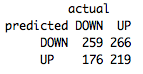About 52%, not bad but let’s see if we can do better.

						TestPredictions<-predict(NB,Test,type="class")


						#Get a list of all our predictions

					

						TestCorrect<-ifelse(TestPredictions==Test[,4],"Correct","Incorrect")


						#See if these predictions are correct

					

						TestData<-data.frame(Test,TestPredictions,TestCorrect)


						#Build one data set we can use for all of our plots

					

Okay, let’s see what patterns our algorithm was able to pick up over the training set and how well those patterns held up over the test set.

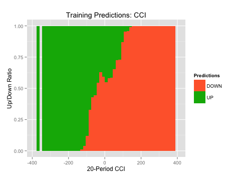
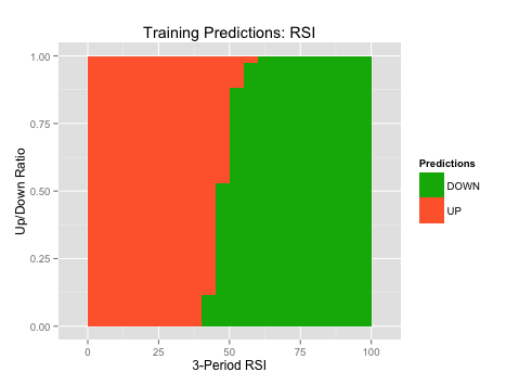
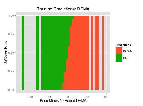
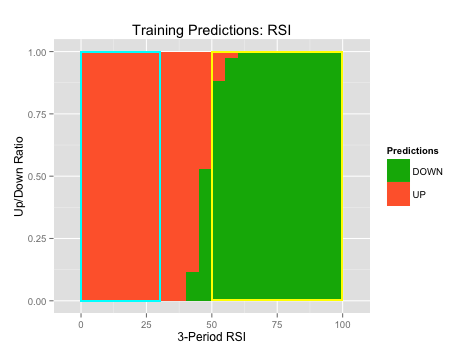
The plots on the left (“Predictions over Training Set”) show where the Naive Bayes algorithm predicted long vs. short over the entire range of our indicator’s values (x-axis). Green is where the algorithm predicted long and orange is where the algorithm predicted short. This allows to see where the algorithm found the strongest long and short signals.

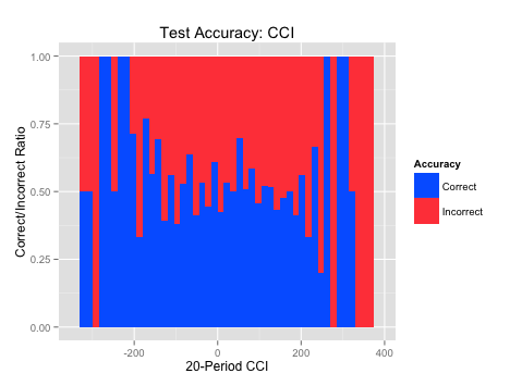
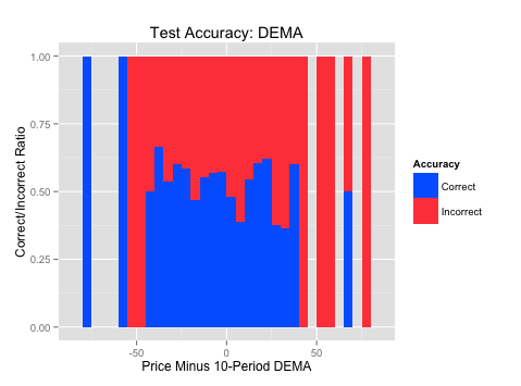
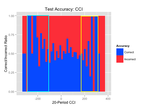
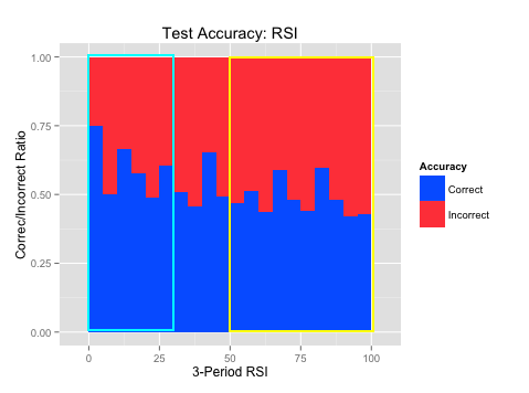
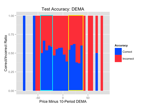
The plots on the right (“Accuracy over Test Set”) show where the algorithm was most accurate across those same indicator values over the test set. Blue is where the algorithm was correct and red is where the algorithm was incorrect over the indicator values (x-axis). This shows us where the patterns best held up over out-of-sample testing. It is always important to test over data the algorithm hasn’t seen to evaluate where it was most accurate.

**Hover over the pictures to enlarge them. Sorry mobile users.

Predictions over Training Set	Accuracy over Test Set

Example code for producing these plots:

Training Predictions:

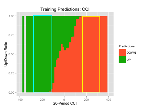
	ggplot(TrainingData,aes(x=CCI20,fill=TrainingPredictions))+geom_histogram(binwidth=15,position="fill")+labs(title="Training Predictions: CCI", x = "20-Period CCI", y= "Up/Down Ratio",fill="Predictions")+scale_fill_manual(values=c("#FF6737","#00B204"))

					

Test Accuracy:

			ggplot(TestData,aes(x=RSI3,fill=TestCorrect))+geom_histogram(binwidth=5,position="fill")+labs(title="Test Accuracy: RSI", x = "3-Period RSI", y= "Correct/Incorrect Ratio",fill="Accuracy")+scale_fill_manual(values=c("#0066FF","#FF4747"))

					

Constructing Your Rules

Great! We have the patterns that our algorithm was able to find in our indicators and how well those patterns held up over new data.

What we want to do now is find the indicator values where 1) the algorithm found a strong buy or sell signal and 2) where the algorithm was more accurate. This will allow us to isolate the values for each indicator where there were both a strong signal and an accurate one. These indicator values then form our rules.

For example, looking at the 20-period CCI, we see that when the indicator value was between -100 and -290, the algorithm found both a strong buy signal and was very accurate. This shows us that this range of indicators should be one of the rules in our long strategy.

The indicator values, and subsequent rules, are highlighted in light blue for long trades and yellow for short trades.

*Note: many machine-learning algorithms are very good at picking up relationships between indicators. For example, it might find that when the CCI is below -200 AND the RSI is below 25, it’s actually a very strong sell signal. However, the Naive Bayes is not one of these algorithms. The term “Naive” actually refers to this, as the algorithm makes the naive assumption that each input is completely independent from the others. So we are analyzing each indicator on its own.

First, we will find the areas where we were able to find strong buy or sell signals. The indicator values, and subsequent rules, are highlighted in light blue for long signals and yellow for short signals. Then, we will find the areas where the algorithm was accurate and it was within the strong buy or sell ranges. Again, the indicator values, and subsequent rules, are highlighted in light blue for long signals and yellow for short signals.

Predictions over Training Set	Accuracy over Test Set

We can then write out the indicator values we isolated into both long and short rules.

Long Rules	Short Rules
IF The CCI20 is above -290 and below -100 AND The RSI3 is below 30 AND The DEMA10cross is above -40 and below -20 THEN Long Signal	IF The CCI20 is above 185 and below 325 AND The RSI3 is above 50 AND The DEMA10cross is above 10 and below 40 THEN Short Signal

Which we then need to test over our validation set:

						Long<-which(Validation$RSI3 < 30 & Validation$CCI > -290 & Validation$CCI < -100 & Validation$DEMA10c > -40 & Validation$DEMA10c < -20)


						#Isolating the trades

					

						LongTrades<-Validation[Long,]


						#Creating a dataset of those trades

					

						LongAcc<-ifelse(LongTrades[,4]=="UP",1,0)


						#Testing the accuracy

					

						(sum(LongAcc)/length(LongAcc))*100


						#And our long accuracy

					

						Short<-which(Validation$DEMA10c > 10 & Validation$DEMA10c < 40 & Validation$CCI > 185 & Validation$CCI < 325 & Validation$RSI3 > 50)

					

						ShortTrades<-Validation[Short,]

					

						ShortAcc<-ifelse(ShortTrades[,4]=="DOWN",1,0)

					

						(sum(ShortAcc)/length(ShortAcc))*100


						#Our short accuracy

					

Leading to our final statistics

 

						length(LongAcc)+length(ShortAcc)


						#Total number of trades

					

 

						((sum(ShortAcc)+sum(LongAcc))/(length(LongAcc)+length(ShortAcc)))*100


						#Total accuracy

					

So we had 46 total trades (a trade about once every 3 days over a 153 day period), with 59% accuracy.

We were able to start with just a broad theory about which indicators are important and very quickly see if there were any patterns in those indicators, and where the strongest and most accurate signals were located. While this is not a huge sample size, it does look like the basis of a good strategy.

Association rule learning allows you to create high-confidence strategies by basing your strategy on mathematically-supported patterns found by our Naive Bayes algorithm and using two out-of-sample tests to make sure those patterns hold up.

We are able to get the benefits of using a machine-learning algorithm, while still understanding the underlying logic of the strategy and easily being able to apply these rules to our own trading.

With TRAIDE, you will be able to easily test a wide variety of inputs and interactively explore, test, and build your own strategy, without needing to spend any time in R. Pre register now to get access as soon as we release!