

Bollinger Bands are one of the more popular technical indicators with many traders using them to both trade the range as well as look for breakouts. However, what features and values should you really be looking at when you are using Bollinger Bands to trade?
In this article we will use a random forests, a powerful machine learning approach, to find what aspects of the Bollinger Bands are most important to a GBP/USD strategy on 4-hour charts.
Bollinger Bands, a technical trading tool developed by John Bollinger in the early 1980s, provide a relative measure of the range of the market. During times of high volatility the trading range will naturally be larger, while in times of low volatility the range will be smaller.
Bollinger Bands are a combination of three lines. The middle line is a simple moving average (usually 20 periods) with the upper line being 2 standard deviations of the close above the middle line and and the lower line being 2 standard deviations below the middle line.
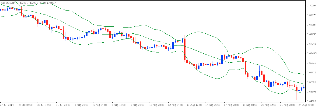
Higher volatility will lead to larger standard deviations and therefore a wider range between the upper and lower bands.
When using the Bollinger Bands in any sort of systematic strategy, the three different lines present some questions and issues; namely, what single factor should you include? Do you want to look at where the current price is relative to the range? Maybe you are only concerned with the upper band for short trades and the lower band for long trades, or do you want to look at the total height of the range?
There are huge number of different values you could look at and this process, known as “feature” selection in the machine learning world, is incredibly important.
Choosing the correct feature that contains the most information relevant to your strategy can have a huge impact on the performance of your strategy.
Instead of needing to evaluate these features yourself, we can use a random forest, a powerful machine learning technique, to objectively evaluate these features for us.
Random forests are an ensemble approach that are based off the principle that a group of “weak learners” can be combined to form a “strong learner”. Random forests start with building a large number of individual decision trees.
Decision trees enter an input at the top of the “tree” and send it down its branches, where each split represents varying levels of indicator values. (To learn more about decision trees, take a look at our previous post where we used a decision tree to trade Bank of America stock.)
Here’s the decision tree we built in a previous post:
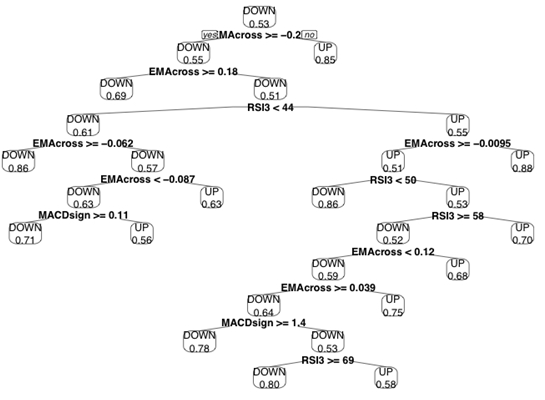
Individual decision trees are seen as fairly weak learners, meaning they can very easily overfit the data and have trouble generalizing well to new data. Combined into “forests” with thousands of “trees”, these simplistic algorithms can form a very powerful modelling approach.
The success on a random forest is derived largely from the ability to create large amount of variability among the individual trees. This is accomplished by introducing a degree of randomness in two different ways:
From these two sources of randomness we have created an entire forest of diverse trees. Now for each data point, each tree is called to make a classification and a majority vote decides the final decision.
One major advantage of random forests is they are able to give a very robust measure of the performance of each indicator. With thousands of trees each built with a different bagged training set and subset of indicators, they tell which indicators were most important in deciding the class of the variable we are trying to predict, in this case the direction of the market.
We take advantage of this valuable property of random forests to figure out which features, derived from the Bollinger Bands, we should be using in our strategy.
First we have to decide what features to derive from the Bollinger Bands. This an area where you can get creative in coming up with fancy calculations and formulas but for now we’ll stick to 8 basic features:
Let’s also look at the percent change of each of the features to add a temporal aspect:
Now that we have our 8 features, let’s build our random forest to see which features we should be using in our strategy.
First let’s install the packages and import our data set (you can download the data used here):
						install.packages(‘quantmod’)

						library(quantmod) #We will use the quantmod package to calculate the Bollinger Bands
						install.packages(‘randomForest’)

						library(randomForest) #The random forest package we will use
DateTime<-as.POSIXlt(GBPUSD[,1],format="%m/%d/%y %H:%M") #format our date and time
HLC<-GBPUSD[,3:5] #Grab the High, Low, Close
						HLCts<-data.frame(HLC,row.names=DateTime)

						HLCxts<-as.xts(HLCts) #Create a timeseries object
Bollinger<-BBands(HLCxts,n=20,SMA,sd=2) #Calculate the bollinger bands
						Upper<-Bollinger$up - HLCxts$Close #Build our first 3 features

						Lower<-Bollinger$dn - HLCxts$Close

						Middle <- Bollinger$mavg - HLCxts$Close
						PChangepctB<-Delt(Bollinger$pctB,k=1) #We’ll use quantmod’s ‘Delt’ function to calculate the percent change

						PChangeUpper<-Delt(Upper,k=1)

						PChangeLower<-Delt(Lower,k=1)

						PChangeMiddle<-Delt(Middle,k=1)
Returns<-Delt(HLCxts$Close,k=1); Class<-ifelse(Returns>0,"Up","Down") #Calculate the percent change and the resultant class we are looking to predict, either an upward or downward move in the market
ClassShifted<-Class[-1] #Shift our class back one since this is what we are trying to predict
Features<-data.frame(Upper, Lower, Middle, Bollinger$pctB, PChangepctB, PChangeUpper, PChangeLower, PChangeMiddle) #Combine all of our features
FeaturesShifted<-Features[-5257,] #Match up with our class
ModelData<-data.frame(FeaturesShifted,ClassShifted) #Combine our two data sets
FinalModelData<-ModelData[-c(1:20),] #Remove the instances where the indicators are being calculated
colnames(FinalModelData)<-c("pctB","LowerDiff","UpperDiff","MiddleDiff","PChangepctB","PChangeUpper","PChangeLower","PChangeMiddle","Class") #Name the columns
set.seed(1) #Set the initial random seed to help get reproducible results
Before we can build our random forest, we need to find the optimal number of indicators to use for each individual tree. Luckily, the random forest package we are using can help us out:
FeatureNumber<-tuneRF(FinalModelData[,-9],FinalModelData[,9],ntreeTry=100, stepFactor=1.5,improve=0.01, trace=TRUE, plot=TRUE, dobest=FALSE) #We are evaluating the features (columns 1 through 9) using the class (column 9) to find the optimal number of features per tree

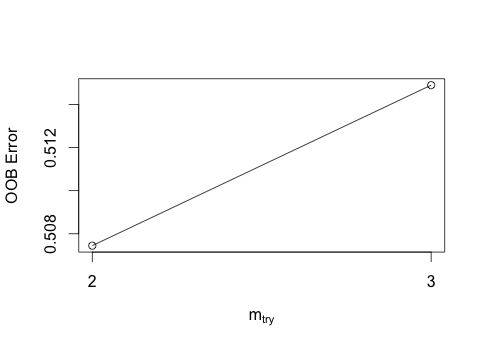
We can see that a tree with 2 features (mtry = 2), had a lower out-of-bag (OOB) error rate so we will go with that for our random forest.
RandomForest<-randomForest(Class~.,data=FinalModelData,mtry=2,ntree=2000,keep.forest=TRUE,importance=TRUE) #We are using all of the features to predict the class, with 2 features per tree, a forest of 2,000 trees, keeping the final forest and we want to measure the importance of each feature. Note: this may take a couple minutes to run.
Let’s see how the features stack up.
varImpPlot(RandomForest)
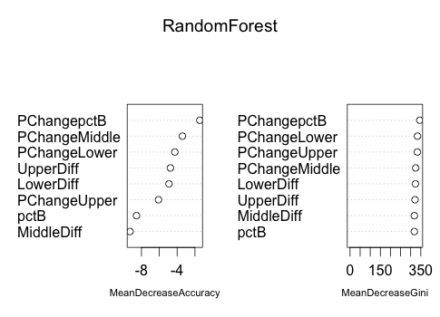
The “mean decrease accuracy” measures how worse each model performs without each feature and the “mean decrease Gini” is a more complex mathematical function that is a measure of how pure the end of each tree branch is for each feature.
We can immediately see that the percent change in the %B value was the most important factor and, in general, looking at the percent change in the values were better than looking at only the distance between the price and the upper, lower, and middle lines.
(Due to the two sources of randomness, you may get slightly different results but overall I found the conclusions to be consistent.)
So now we know what features, based on the Bollinger Bands, we should use in our trading strategy.
Random forests are a very powerful approach that commonly outperform more sophisticated algorithms. They can be used for classification (predicting a category), regression (predicting a number), or with feature selection (like we saw here).
Feature selection, or deciding what factors to include in your strategy, is an incredibly important part of building any strategy and there are many techniques in machine learning focused on solving this problem.
With TRAIDE, we take care of the second step: once you have selected the features for your strategy, we use machine-learning algorithms to find the patterns for you.
Create your own account here and, as always, happy TRAIDING!