

Machine-learning algorithms can be used to find the best values to trade your indicators.
The Relative Strength Index, or RSI, is one of the most common technical indicators. It is used to identify oversold and overbought conditions. Traditionally, traders look for RSI values over 70 to represent overbought market conditions and under 30 to represent oversold market conditions. However, is there any validity to these claims? Why 70 and why 30? Further, how do different trending markets affect the RSI signals you should be looking for?
In this post, we’ll use a Support Vector Machine (SVM), a powerful machine-learning algorithm, to explore what values of an RSI you should actually be looking for while taking into account the overall trend in the market.
First, we’ll give a brief overview of the SVM, then outline the problem, and finally build and test a strategy based off of the patterns discovered by the algorithm.
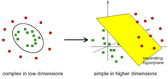
Support Vector Machines are one of the more popular and powerful “off-the-shelf” machine-learning algorithms based on their ability to find non-linear patterns. SVMs work by finding a line, known as a “decision boundary” or “hyperplane”, that best separates your data based on the class (in our case, “bullish” or “bearish” bars). The power of an SVM is being able to rearrange, or map, your data with a set of mathematical functions, known as “kernels”, into a multidimensional feature space where your data is linearly separable.

The SVM then draws a line in the higher dimensional space that maximizes the distance between the two classes. When a new data point is presented to the SVM, it then calculates which side of the line the point falls and makes its prediction.
Another advantage of the SVM is there are relatively few parameters that must be selected before you are able to use it. First, you must select the kernel, or mapping, function to use to translate your data into a higher dimensional space. A radial basis function is a popular choice and will work well in our case. Next, you need to choose the gamma parameter. The gamma determines how much effect a single training example can have on the decision boundary. Low values mean a single point will have a large effect on where the line is drawn and high values mean each point will only have a small effect. A good rule of thumb to select the gamma parameter to be one over number of inputs to your model (1/(number of inputs)). Finally, you need to choose the regularization parameter, C. C determines the trade off between misclassifying examples in your training set and the simplicity of the decision boundary. A low C creates a smoother decision boundary and decreases overfitting, while a high C will attempt to classify every data point in the training set correctly and may lead to overfitting. We want to decrease how much our model overfits so we will select a value of 1 but feel free to play around with it yourself.
Now that we have a basic idea of how a Support Vector Machine works and how to select its parameters, let’s see if we can use it to figure out how to trade an RSI.
The relative strength index, or RSI, compares the average size of the “up” moves to the average size of the “down” moves and normalizes it between 0 and 100. The conventional logic goes that once the asset has had more, significant upticks, it has become overbought, or overvalued, and is likely to decrease in price. Overbought is usually determined by an RSI value over 70, with opposite conditions representing oversold, or undervalued, at an RSI value of 30.
However, these conditions don’t happen in a vacuum. There are also broader market trends at work. An RSI value over 70 in the middle of a strong uptrend might represent a continuation of the trend while a value of 70 during a downtrend could signify a great entry point. The problem is finding out exactly what conditions we should be looking for considering both factors.
We could gather thousands of data points and try to find those relationships ourselves or we could use a Support Vector Machine, an algorithm designed to find non-linear patterns, to do the legwork for us.
Let’s see what patterns we are able to find in a 3-period RSI and define a trend by comparing the open price to a 50-period simple moving average (SMA) using the AUD/USD 4 hour charts.
Let’s use R to build our model, analyze the patterns it was able to find and then test to see if those patterns hold up in an actual trading strategy.
						install.packages(“quantmod”)

						library(quantmod)

						#A great quantitative trading resource
						install.packages(“e1071”)

						library(e1071)

						#The library containing our SVM
						install.packages(“ggplot2”)

						library(ggplot2)

						#The plotting tools we will use
To create the data set and build the model:
						Data<-AUD/USD

						#Our 4-hour bars of the Australian Dollar/US Dollar currency pair dating back to 01/01/2010. You can download it here (dropbox) for your own use.
						RSI3<-RSI(Op(Data),n=3)

						#The 3-period relative strength index calculated off the open
						SMA50<-SMA(Op(Data),n=50)

						Trend<-Op(Data)-SMA50

						#Our measure of trend: the difference between the open price and the 50-period simple moving average
						Price<-Cl(Data)-Op(Data)

						Class<-ifelse(Price>0,"UP","DOWN")

						#The variable we are looking to predict; the direction of the next bar
						DataSet<-data.frame(RSI3,Trend,Class)

						DataSet<-DataSet[-c(1:49),]

						#Create the data set and removing the points where our indicators are still being calculated
						Training<-DataSet[1:4528,]

						Test<-DataSet[4529:6038,]

						Val<-DataSet[6039:7548,]

						#Separate the data into 60% training set to build our model, 20% test set to test the patterns we found, and 20% validation set to run our strategy over new data
						SVM<-svm(Class~RSI3+Trend,data=Training, kernel="radial",cost=1,gamma=1/2)

						#Build our support vector machine using a radial basis function as our kernel, the cost, or C, at 1, and the gamma function at ½, or 1 over the number of inputs we are using
						TrainingPredictions<-predict(SVM,Training,type="class")

						#Run the algorithm once more over the training set to visualize the patterns it found
						TrainingData<-data.frame(Training,TrainingPredictions)

						#Create a data set with the predictions
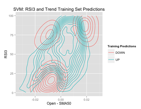
						ggplot(TrainingData,aes(x=Trend,y=RSI3))+stat_density2d(geom="contour",aes(color=TrainingPredictions))+labs(title="SVM RSI3 and Trend Predictions",x="Open - SMA50",y="RSI3",color="Training Predictions")

						#Now let’s see what patterns it was able to find

Interesting! We can see three distinct areas where the algorithm went short and one range in the middle where it only went long. Let’s explore further.
| Long | Short |
|---|---|
| RSI below 25 and the Price is more than 20 pips below the SMA 50 (56% accurate, 36 trades) | RSI less than 25 and the Price is between 10 and 5 pips below the SMA 50 (54% accurate, 81 trades) |
| RSI3 is between 50 and 75 and the Price is between 5 and 10 pips above the SMA 50 (58% accurate, 104 trades ) | RSI greater than 70 and the Price more than 5 pips below the SMA 50 (59% accurate, 37 trades) |
| RSI greater than 75 and price more than 15 pips above the SMA 50 (59% accurate, 34 trades) |
First the short area on the bottom left. Here the price has just crossed below the 50-period SMA and the RSI is below 25, suggesting a breakout of a downward trend.
However, if the price moves beyond 20 pips below the 50-period SMA and the RSI remains under 25, the algorithm found a stronger signal for a reversion to the mean and predicted a long trade.
Next, the short opportunity on the upper left of the plot represents the traditional view of the RSI. Here we are looking for the RSI to be over 70 while the price is more than 15 pips above the 50-period SMA to represent “overbought” conditions, suggesting we go short.
The short area on the upper left is a little different. When the price had just crossed below the 50-period SMA and the RSI was over 70, it found a short opportunity. This is similar to the first case but instead of traditional “overbought” conditions, we are looking for a bearish breakout entry signal.
Finally, there was an area where the RSI was between 50 and 75, while the price had crossed above the 50-period SMA where the algorithm found a strong buy signal.
Now that we have found a basic set of rules that the SVM uncovered, let’s test to see how well they hold up over new data, our test set.
ShortRange1<-which(Test$RSI3 < 25 & Test$Trend > -.010 & Test$Trend < -.005)
ShortRange2<-which(Test$RSI3 > 70 & Test$Trend < -.005)
ShortRange3<-which(Test$RSI3 > 75 & Test$Trend > .015)
LongRange1<-which(Test$RSI3 < 25 & Test$Trend < -.02)
LongRange2<-which(Test$RSI3 > 50 & Test$RSI3 < 75 & Test$Trend > .005 & Test$Trend < .01)
Now let’s see how well these patterns hold up over out test set:
						ShortTrades<-Test[c(ShortRange1,ShortRange2,ShortRange3),]

						ShortCorrect<-((length(which(ShortTrades[,3]=="DOWN")))/nrow(ShortTrades))*100

						#Our short trades
						LongTrades<-Test[c(LongRange1,LongRange2), ]

						LongCorrect<-((length(which(LongTrades[,3]=="UP")))/nrow(LongTrades))*100

						#Our long trades
Wow! 58% (85 correct out of 147 trades) for our short trades and 57% (80 correct out of 140 trades) for our long trades.
Now let’s turn this into an actual trading strategy with a stop loss and take profit as our exit conditions.
[Note: see my previous post “How to Backtest in R” for step-by-step instructions]
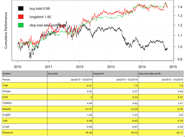
I added a fairly tight take profit and stop loss and maintained a 1:1 risk-to-reward ratio due to the short nature of our predictions (just one bar) and to take advantage of our over 50% accuracy.
Let’s see how well we did:

You can see how well the strategy did compared to the a buy-and-hold strategy and just the entry signals. Overall, the equity curve looks fairly smooth and a strategy based off these two simple indicators looks very promising.
Using a Support Vector Machine, a powerful machine-learning algorithm, we were not only able to learn under what conditions the conventional wisdom of an RSI hold up but we were able to create a robust trading strategy.
This process, known as Association Rule Learning, or deriving rules from machine-learning algorithms, allows you to leverage the capabilities of a machine-learning algorithm with your own experiences as a trader.
We believe that the best results are found when combining both man and machine, and this has formed the basis of TRAIDE. We are excited to announce that TRAIDE for FX is now available so sign up now for a free trial. We’d love to have your feedback!