


We're going to explore the backtesting capabilities of R.
In a previous post we developed some simple entry opportunities for the USD/CAD using a machine-learning algorithm and techniques from a subset of data mining called association rule learning. In this post, we are going to explore how to do a full backtest in R; using our rules from the previous post and implementing take profits and stop losses.
Let's dive right in:
						library(RCurl)


						library(quantmod)


						#Install the libraries we need
						sit = getURLContent('https://github.com/systematicinvestor/SIT/raw/master/sit.gz', binary=TRUE, followlocation = TRUE, ssl.verifypeer = FALSE)


						con = gzcon(rawConnection(sit, 'rb'))


						source(con)


						close(con)


						#Download Michael Kapler's “Systematic Investor Toolbox”, a powerful set of tools used to backtest and evaluate quantitative trading strategies
						data <- new.env()


						#Create a new environment
						tickers<-spl('USDCAD')


						file.path<- ‘my.file.path’


						#Specify the name of the asset and where the csv file is located on your computer. (You can find more ways to load data here.)
						for(n in tickers) { data[[n]] = read.xts(paste(file.path, n, '.csv', sep=''), format='%m / %d / %y %H:%M') }


						bt.prep(data, align='remove.na')


						#Load and clean the data
						prices = data$prices


						models = list()


						#Specify the prices and store our models
						data$weight[] = NA


						data$weight[] = 1


						models$buy.hold = bt.run.share(data, clean.signal=T)


						#Create our baseline “Buy and Hold” strategy
						CCI20<-CCI(prices,20)


						RSI3<-RSI(prices,3)


						DEMA10<-DEMA(prices,n = 10, v = 1, wilder = FALSE)


						DEMA10c<-prices - DEMA10


						DEMA10c<-DEMA10c/.0001


						#Calculate the indicators we need for our strategy
						buy.signal<-ifelse(RSI3 < 30 & CCI20 > -290 & CCI20 < -100 & DEMA10c > -40 & DEMA10c < -20,1,NA)


						#Set our long entry conditions found by our algorithms and optimized by us in the last post
						data$weight[] = NA


						data$weight[] = buy.signal


						models$long = bt.run.share(data, clean.signal=T, trade.summary = TRUE)


						#Create our long model
						sell.signal<-ifelse(DEMA10c > 10 & DEMA10c < 40 & CCI20 > 185 & CCI20 < 325 & RSI3 > 50, -1 ,NA)


						#Set our short conditions
						data$weight[] = NA


						data$weight[] = sell.signal


						models$short = bt.run.share(data, clean.signal=T, trade.summary = TRUE)


						#Create our short model
						long.short.strategy<-iif(RSI3 < 30 & CCI20 > -290 & CCI20 < -100 & DEMA10c > -40 & DEMA10c < -20,1,iif(DEMA10c > 10 & DEMA10c < 40 & CCI20 > 185 & CCI20 < 325 & RSI3 > 50, -1 ,NA))


						#Set the long and short conditions for our strategy
						data$weight[] = NA


						data$weight[] = long.short.strategy


						models$longshort = bt.run.share(data, clean.signal=T, trade.summary = TRUE)


						#Create our long short strategy
						dates = '2014-02-26::2014-09-22'


						#Isolate the dates from our validation set (The data not used to train the model or create the rules, our out-of-sample test)
bt.stop.strategy.plot(data, models$longshort, dates = dates, layout=T, main = 'Long Short Strategy', plotX = F)Note: the backtest is built off the 4-hour bars in our data set and doesn’t have a more granular view.
#View a plot of our trades

						strategy.performance.snapshoot(models, T)


						#View the equity curve and performance statistics.
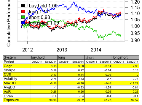
The CAGR (compounded annual growth rate) is the percentage gain/loss annualized, meaning it smooths out the growth into equal instalments each year. Since our test was over Let’s see if we can improve the performance by adding a stop loss and take profit.
						stop.loss <- function(weight, price, tstart, tend, pstop) {


						index = tstart : tend


						if(weight > 0)


							price[ index ] < (1 - pstop) * price[ tstart ]


						else


							price[ index ] > (1 + pstop) * price[ tstart ]


						}


						#The stop loss function
						Stoploss = .25/100


						#Set our maximum loss at a .25% move in price against our trade
						data$weight[] = NA


						data$weight[] = custom.stop.fn(coredata(long.short.strategy), coredata(prices), stop.loss,pstop = Stoploss)


						models$stoploss = bt.run.share(data, clean.signal=T, trade.summary = TRUE)


						#Our long short model with a .25% stop loss
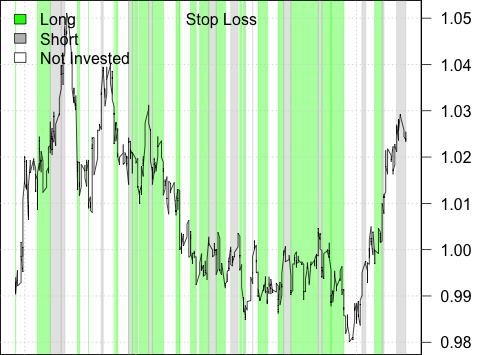
						bt.stop.strategy.plot(data, models$stoploss, dates = dates, layout=T, main = 'Stop Loss', plotX = F)

						#The plot of our trades
						strategy.performance.snapshoot(models[c(1,4:5)], T)

						#And how it compares to the original model

With just a stop loss, performance went down. It looks like we are getting taken out of our trades before they are able to recover. In order to lock in our profits, let’s go ahead and implement a take profit.
						take.profit<- function(weight, price, tstart, tend, pprofit) {


							index = tstart : tend


							if(weight > 0)


								price[ index ] > (1 + pprofit) * price[ tstart ]


							else


								price[ index ] < (1 - pprofit) * price[ tstart ]


							}


						#The take profit function
						Takeprofit = .25/100


						#Maintain at 1:1 risk/reward ratio and set our take profit at a .25% change in price
						data$weight[] = NA


						data$weight[] = custom.stop.fn(coredata(long.short.strategy), coredata(prices), take.profit, pprofit = Takeprofit)


						models$takeprofit = bt.run.share(data, clean.signal=T, trade.summary = TRUE)


						#Our long short model with a .25% take profit
						bt.stop.strategy.plot(data, models$takeprofit, dates = dates, layout=T, main = 'Take Profit', plotX = F)


						#The plot of our trades

						strategy.performance.snapshoot(models[c(1,4:6)], T)

						#Compare it to our other models
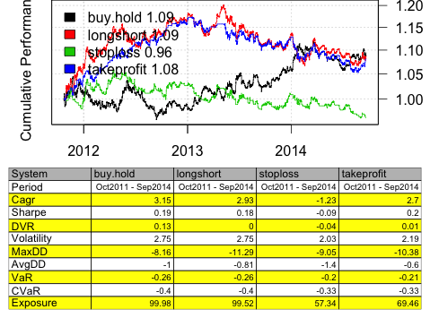
Locking in our gains with a take profit slightly improved the performance, but not drastically. Let’s incorporate both a stop loss and a take profit.
						stop.loss.take.profit<-function(weight, price, tstart, tend, pstop, pprofit) {


							index = tstart : tend


							if(weight > 0) {


								temp = price[ index ] < (1 - pstop) * price[ tstart ]


								# profit target


								temp = temp | price[ index ] > (1 + pprofit) * price[ tstart ]


							} else {


								temp = price[ index ] > (1 + pstop) * price[ tstart ]


								# profit target


								temp = temp | price[ index ] < (1 - pprofit) * price[ tstart ]


							}


							return( temp )


						}


						#The stop loss and take profit function
						data$weight[] = NA


						data$weight[] = custom.stop.fn(coredata(long.short.strategy), coredata(prices), stop.loss.take.profit,pstop = Stoploss, pprofit = Takeprofit)


						models$stop.loss.take.profit = bt.run.share(data, clean.signal=T, trade.summary = TRUE)


						#Our long short model with a .25% stop loss and .25% take profit
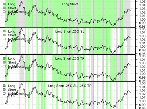
Now let’s compare the baseline Long Short strategy, with just a stop loss, just a take profit, and both a take stop loss and take profit.
						layout(1:4)


						bt.stop.strategy.plot(data, models$longshort, dates = dates, layout=T, main = 'Long Short', plotX = F)


						bt.stop.strategy.plot(data, models$stoploss, dates = dates, layout=T, main = 'Long Short .25% SL', plotX = F)


						bt.stop.strategy.plot(data, models$takeprofit, dates = dates, layout=T, main = 'Long Short .25% TP', plotX = F)


						bt.stop.strategy.plot(data, models$stop.loss.take.profit, dates = dates, layout=T, main = 'Long Short .25% SL, .25% TP', plotX = F)


						#The plot of our trades
						strategy.performance.snapshoot(models[c(1,4:7)], T)


						#Finally comparing all the models we created

Now you know how to add a take profit and stop loss, I recommend you play around with the data and test different values based on your own personal risk parameters and using your own rules.
Even with powerful algorithms and sophisticated tools, it is difficult to build a successful strategy. For every good idea, we tend to have many more bad ones. Armed with the right tools and knowledge, you can efficiently test your ideas until you get to the good ones. We have streamlined this process in TRAIDE. We’ve developed a testing infrastructure that allows you to see where the patterns are in your data are and in real-time see how they would have performed over your historical data.
We’ll be releasing TRAIDE for 7 major pairs in the FX market with technical indicators in two weeks. If you are interested in testing the software and providing feedback, please send an email to info@inovancetech.com. We have 50 spots available.