

Selecting the indicators to use is one of the most important and difficult aspects of building a successful strategy.
Not only are there thousands of different indicators, but most indicators have numerous settings which amounts to virtually limitless indicator combinations. Clearly testing every combination is not possible, so many traders are left on their own selecting somewhat random inputs to build their strategy.
Luckily this process, known as “feature selection”, is a very well-researched topic in the machine learning world. In this post we’ll use a popular technique known as a “wrapper method” that uses a support vector machine (SVM) and a “hill climbing” search to find a robust subset of indicators to use in your strategy.
Selecting from the near limitless possible combinations of indicators to use in your strategy can be very daunting. However, this is a problem that machine learning experts and data scientists have been grappling with for a long time and have come up with a wide range of tools and techniques to help you out.
One popular technique is a wrapper method. A wrapper method uses a machine-learning algorithm to evaluate each subset of indicators. The main advantage to this method, as opposed to evaluating each indicator on its own, is we can find the relationships and dependencies between indicators. For example, a 14-period RSI or a 30-period CCI alone may not be great predictors, but combined could provide some valuable insight.
The next question is how do you decide which subsets of indicators to evaluate? If you are only looking at a few indicators then trying every combination might be possible, but even looking through 15 different indicators for 3 to use in your strategy leads to over 450 different possible combinations! Other techniques either rank the indicators based on a certain performance metric, like correlation, or start with the full or empty set and add/subtract indicators one by one. These type of searches are known as being “greedy”, meaning that they can only search in one direction, e.g. going from strongest correlation to weakest, but may miss some important relationships between indicators.
One method that attempts to get around this is the known as a “hill climbing” method. A hill climbing method starts with a random subset of indicators and then evaluates all of the “neighboring” combinations, selecting the best performing combination. While this does allow us to find interesting relationships between indicators, there is a chance that we get stuck in what’s called a “local maximum,” which means that it may just be the best combination of neighbors but not necessarily the best overall combination. To get around this, we can run the search multiple times to see what patterns emerge in the top neighboring subsets.
For this article, we’ll use a support vector machine (which we previously used to build a strategy for the RSI) and repeat the hill climbing search 10 times to find the best subset.
Even when using these techniques, we still need to define the feature space to search from. This is where your domain experience comes in. Now you may not know the best period to use, but you most likely have a set of “favorite” indicators that you know and make sense to you conceptually. You can give this process a huge head start by selecting meaningful, relevant indicators that you understand.
In the name of simplicity, we’ll start with just 5 different and commonly used base indicators: SMA, EMA, RSI, CCI and MACD.
We can use different periods and calculations based off these indicators to create features.
For example, here are 20 different "features":
| Price - SMA(5) | Price - SMA(30) |
| Price - SMA(50) | SMA(5) - SMA(30) |
| SMA(5) - SMA(50) | SMA(30) - SMA(50) |
| Price - EMA(5) | Price - EMA(30) |
| Price - EMA(50) | EMA(5) - EMA(30) |
| EMA(5) - EMA(50) | EMA(30) - EMA(50) |
| RSI(5) | RSI(14) |
| RSI(30) | CCI(5) |
| CCI(14) | CCI(30) |
| MACD_Line | MACD_Signal |
We can see how even looking at only 5 indicators leads to a huge number of possible inputs to your strategy!
Let's get started building our model. We'll explore the usefulness of the above 20 features in building a profitable strategy.
Now that we have our features we can build our model in R (When working with an SVM, it is important to normalize the data: You can download the original data and the normalized data we use for inputs to the model here).
First, we need to install the necessary libraries:
						install.packages(“FSelector”) # the library for the hill climbing search

						library(FSelector)

						install.packages(“e1071”) # the library for the support vector machine

						library(e1071)

						install.packages(“ggplot2”) # the library for our plots

						library(ggplot2)
Then split the data into our training and test sets. We’ll use ⅔ of the data to build the model and reserve ⅓ to test out of sample.
						Breakpoint <- nrow(Model_Data)*(2 / 3)

						Training<-Model_Data[1:Breakpoint, ]

						Validation<-Model_Data[(Breakpoint+1):nrow(Model_Data), ]
We’ll then need to build the function that evaluates each subset using the SVM. We’ll break our training set into another training and test set to evaluate these models on data that was not used in the building process. This is another check to make sure we are not overfitting.
					SVM_Evaluator<-function(subset){

					data<-Training

						break_point<-(2/3)*nrow(data)

						Training_Set<-data[1:break_point,]

						Test_Set<-data[(break_point+1):nrow(data),]

						SVM<-svm(Predicted_Class~.,data=Training_Set, kernel="radial",cost=1,gamma=1/20)

						SVM_Predictions<-predict(SVM,Test_Set,type="class")

						Accuracy<-sum(SVM_Predictions == Test_Set$Predicted_Class)/nrow(Test_Set)

						return(Accuracy)

					}
Now we can run the hill climbing search once to see what it finds:
						set.seed(2)

						Attribute_Names<-names(Training)[-ncol(Training)]

						Hill_Climbing<-hill.climbing.search(Attribute_Names,SVM_Evaluator)
But what we really care about is running it 10 times to help stabilize the results (this will take a couple minutes to run):
						set.seed(2)

						Replication_Test <-replicate(10,hill.climbing.search(Attribute_Names,SVM_Evaluator))
Let’s dive into the results and take a look at which indicators tended to be included in the best subsets:
						Indicator_Count<-function(names){

							as.numeric(length(grep(names,Replication_Test)))

							}


						Distribution<-lapply(Attribute_Names,Indicator_Count)

						Attribute_Names_df<-as.data.frame(Attribute_Names)


						Distribution_df<-t(data.frame(Distribution))

						Indicator_Distribution<-data.frame(Attribute_Names_df,Distribution_df,row.names=NULL)


						ggplot(Indicator_Distribution,aes(x=Attribute_Names,y=Distribution_df))+geom_bar(fill="blue",stat="identity")+ theme(axis.text.x = element_text (size=10,angle=90,color="black"), axis.title.x=element_text(size=15),axis.title.y=element_text(size=15),title=element_text(size=20))+labs(y="Appearances in Subsets",x="Indicator Name",title="Indicator Subset Frequency")+ylim(c(0,10))

Interesting, so we can see that the distance between the price and a 5-period simple moving average (“Price_Minus_SMA_5”) appeared in 9 of the 10 subsets, followed by the distance between the price in a 5-period exponential moving average (“Price_Minus_EMA_5”) and the distance between the price in a 50-period exponential moving average (“Price_Minus_EMA_50”) in 8 of the 10 subsets. Since we are looking to predict only the next bar, it makes sense that the shorter periods would perform best but it is interesting that a simple moving average was selected in more subsets than the exponential moving average.
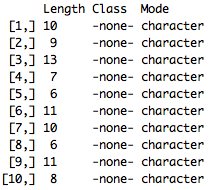
Now let’s see how many indicators are in each subset:
summary(Replication_Test)

So the 5th and 8th iterations of our search each had top subsets with only 6 indicators but while I tend to favor subsets with smaller number of indicators, the 4th iteration was the smallest subset that included our top feature, the “Price_Minus_SMA_5”, so let’s use that one as our final model:
Replication_Test[ [ 4 ] ]
| PRICE_Minus_SMA_5 | PRICE_Minus_SMA_30 | PRICE_Minus_SMA_50 |
| PRICE_Minus_EMA_30 | CCI_5 | CCI_30 |
| MACD_Signal |
We’ll build the final model with the entire Training Set and test it over our yet-to-be-touched Validation set:
						SVM_Final<-svm(Predicted_Class~PRICE_Minus_SMA_5+PRICE_Minus_SMA_30+PRICE_Minus_SMA_50+PRICE_Minus_EMA_30+CCI_5+CCI_30+MACD_Signal,data=Training, kernel="radial",cost=1,gamma=1/20)


						SVM_Predictions_Final<-predict(SVM_Final,Validation,type="class") # Predict over the Validation set


						Accuracy_Final<- Accuracy<-sum(SVM_Predictions_Final == Validation$Predicted_Class) /nrow(Validation)
Very nice, so over our out-of-sample validation set, we were able to get 53% accuracy! While this does not seem like much, the point of this process was to be able to find a robust subset of indicators. Now we have a baseline of 53% accuracy that we can then use to further build and improve our strategy.
With TRAIDE, we can then use an ensemble of machine-learning algorithms to find the most profitable entry signals based on these indicators.
Now it’s your turn to use machine learning to build your next strategy!